Control Theory: Example 3 – P-only control and offset

introduction

I want to see exactly how we get offset under P-only control, and how PI control eliminates the offset. I’m going to use Example 3 again… I’m going to look at P and PI control… and I’m going to use the Tyreus-Luyben (“T-L”) tuning rules, which we’ve seen before.

When I started this, I was wondering about two things:

• Is the control effort nonzero when we have offset?
• We don’t always have offset under P-only control, do we?

I can’t say I’ve become an expert in offset, but I’m a little more comfortable with it. Now what I’d like to know is why the control effort goes to zero when we do not have offset – but that’s a question still looking for an answer.

Let me tell you up front what we will find:

• With P-only control, we may have offset: the output will not tend to the set point.
• In that case, the use of PI-control will eliminate offset.
• But if our plant (G) has a pole of any order at the origin, then P-only control does not lead to offset.
• In that case, you could imagine that the plant itself includes integral control.

Let us recall Example 3. This plant is a 3rd-order transfer function… as usual, rules are a convenient way to specify things:

The plant G, then, has the following transfer function:

I’ve shown you the right way to get the ultimate gain and ultimate period, if you have a quantitative model. Let’s do it again.

We get the open loop Bode plot… start with the open loop transfer function GK:

And here’s the plot:

The first pair of numbers tells us that the gain margin is 10 and that it occurs at a frequency of 1 radian/second. Given a frequency f in radians/second, we find the period from P f = 2 pi. This crossover frequency is 1, so the corresponding period is

That is, the ultimate gain is ku = 10 and the ultimate period is . Now save these:

Now that we have Pu and ku, there are some rules for setting the parameters of P, PI, and PID controllers. But while I have the default K = 1, let’s see how the uncontrolled plant responds to a unit step.

If it helps, think of the uncontrolled plant as nevertheless having K = kc = 1: a P-only controller with gain = 1. It is crucial that the plant response is nonzero – but it seems to have a steady-state value of .5 instead of 1. This is offset.

We can check that directly, by taking the limit as t goes to infinity…

Or we can use the final-value theorem – but remember that the output is the inverse Laplace transform of y/s, so we use s (y/s), which is just y:

Anyway, the plant itself responds… it just doesn’t respond enough. Adding a P-only controller will increase the gain, and will move the long-term response closer to 1.

P-only control

So let’s start by inserting a PID controller:

To get P-only control, we set and . I have a rule for that:

The open loop transfer function, then, is…

Here are the closed loop transfer functions for output and for control…

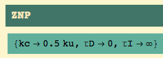
The T-L rule for P-only control is to set kc = .5 ku – the same as the Z-N rule. (Parts of the following rule are redundant, because I’ve already set , but I like having a complete rule anyway.)

So the closed loop output becomes.. and we know the ultimate gain ku:

and the closed loop for control becomes

We get the time-domain responses to a unit step input by taking inverse Laplace transforms of y/s and of u/s…

And we plot the input (step function in “silver” or whatever it is), output (black), and scaled control effort (gold):

Not only does it take a long time to settle, but there is offset. As for the long settling time… K = 1 got there quickly, K = 10 was on the edge of instability, so K = 5 should have decaying oscillations. OK?

For the record, here’s the unscaled control effort (gold):

Let me look at the long-time response – pick it up at t = 30 (and note the numbers on the vertical axis):

Isn’t it interesting that the steady-state control effort is not zero? The controller must be active in order to hold the output away from zero. I infer that if we were to turn of the control (that is. set kp = 1), the system would return to 0.5, its long-term uncontrolled value (i.e. with kp = 1).

Let’s see exactly the long-term values of output…

They’re the same. We’re driving a linear constant-coefficient differential equation with a constant forcing function; because the forcing function = 1, the output is the same constant. We’ve also just seen one very good reason for not scaling the control effort: I missed that it’s equal to the output.

This is the first clue as to how offset can occur: the control effort is not strong enough to push the system to an output of 1.

Let’s look even closer. We’ve seen that the output has offset: we are not at “1”. We’ve seen that the controller does not tend to zero (“off”) in the long term. So just what does the error look like?

Well, the error is input (“reference” or set point) minus output: r – y.

Hmm. The error is very small, but nonzero.

Well, if the control effort is to be nonzero, then the error must be nonzero. Right? Under P-only control, we have that the controller has kc = 5:

and the time-domain formulation is that the control effort is proportional to the error, with a proportionality constant of 5… so let’s compute 5 e:

We need to see that over the entire range:

Compare that to a plot of the unscaled control effort c1:

The same.

OK…. both the error and the control effort tend to nonzero values over time. And the control effort is enough to hold the output significantly away from zero, and actually closer to 1 than without control – but not enough to hold it at 1.

But there is a second issue involved. The ultimate gain for this system is 10 – which means that if we set the controller gain above 10, then the closed system will be unstable.

What happens if we raise the controller gain to 9.9?

P with large gain

So let’s just set K = 9.9

The open loop transfer function is…

Here are the closed loop transfer functions for output and for control…

We get the time-domain responses to a unit step input by taking inverse Laplace transforms of y/s and of u/s…

And we plot the input (step function in “silver”) and output (black):

Well that’s not very informative. Eventually we settle down at a value just over 0.9:

So let’s go way out – start time at 2000:

So we did get closer, but, boy, does it take a long time.

Oh, what’s the control effort? As before, it’s the output value, in this case 0.9 +.

Anyway, the real point – the second issue – is that we can’t raise the gain enough to eliminate offset.

PI-control

Now let’s add integral control. Oh, I need to restore my PID controller:

To get PI control, we set .

The open loop transfer function is…

Here are the closed loops for output and for control…

The T-L rules for PI control are

so the closed loop output becomes.. and we use the ultimate gain ku and ultimate period Pu…

The closed loop for control becomes

The time-domain responses are…

Here is the usual plot showing input, output (black), and scaled controller effort (gold):

It settles faster, and the offset is gone.

After all, that’s one of things integral control does for us: it eliminates offset. I should point out that we don’t always care about offset: level control for surge tanks is the best example where we do not care to hold the level at exactly 50%. In fact, to do so would defeat the purpose of a surge tank, and we might as well replace it by a pipe – where what goes out is exactly what comes in.

Here’s the unscaled control effort:

For the record, we find the long-term limits: both the output and the control effort tend to 1:

As before, let’s look a little closer. With a PI controller, there are two error terms. One is the error itself, and that gives us the P-control. The other, however, is the integrated error, and that’s what gives us the I-control.

OK… The error is e = r – y, i.e.

(I will need a variable of integration, and I don’t want it to be t, because t will be the upper limit on the definite integral. So I need to be able to set the variable for e.)

Since the output tends to 1, we know that the error tends to zero:

What about the integrated error? We integrate from 0 to t, using as the variable of integration:

(The only difference in those two expressions, I think, is that +0.i disappeared as a result of the Chop command.)

As t goes to infinity, the integrated error tends to a constant positive value:

Now, what does the I-term do in the controller? In the time domain, the controller is

i.e. the I-term is… and tends to 1 as time tends to infinity…

Despite all the terms, the key is the two constants at the beginning:

That’s why the control effort tends to 4. whatever.

Two examples without offset

First, forget that we have PI-control on that plant… imagine that we have our latest closed-loop transfer function, and that it represents an uncontrolled system. What is the G that leads to such a closed-loop transfer function?

That is, we find G such that G / (1+G) = y:

Note that G1 has a pole of order 1 at the origin (i.e. s in the denominator).

Given the warning message, let me check that answer. Use the given open-loop G1 and compute its closed-loop transfer function… and compare it to the one we started with:

And what we see is that if we had started with a plant G that had a pole at zero, then P-only control would have worked.

It’s an interesting game, and I’m sure I’ll be playing it again: usually, set the closed-loop response and the system G, and find the controller K to get the desired closed-loop.

Let me try something simpler. Let’s just take 1/s for the system, and compute the closed-loop transfer function:

Now get the output and control effort in response to a unit step input:

Interesting. Very interesting: the control effort goes to zero… as the error goes to zero… and we do not have offset.

So. As I said at the beginning:

• With P-only control, we may have offset: the output will not tend to the set point.
• In that case, the use of PI-control will eliminate offset.
• But if our plant (G) has a pole of any order at the origin, then P-only control does not lead to offset.
• In that case, you could imagine that the plant itself includes integral control.

Let me be blunt. It would be wrong to say that P-only control always leads to offset.