Control Theory: Example 3 – P-only control and offset

introduction

I want to see exactly how we get offset under P-only control, and how PI control eliminates the offset. I’m going to use Example 3 again… I’m going to look at P and PI control… and I’m going to use the Tyreus-Luyben (“T-L”) tuning rules, which we’ve seen before.

When I started this, I was wondering about two things:

• Is the control effort nonzero when we have offset?
• We don’t always have offset under P-only control, do we?

I can’t say I’ve become an expert in offset, but I’m a little more comfortable with it. Now what I’d like to know is why the control effort goes to zero when we do not have offset – but that’s a question still looking for an answer.

Let me tell you up front what we will find:

• With P-only control, we may have offset: the output will not tend to the set point.
• In that case, the use of PI-control will eliminate offset.
• But if our plant (G) has a pole of any order at the origin, then P-only control does not lead to offset.
• In that case, you could imagine that the plant itself includes integral control.

The Economic Order Quantity – a simple calculus application

The EOQ (Economic Order Quantity) formula is a deceptively simple model. It comes from Zipkin’s “Foundations of Inventory Management” (Irwin/McGraw-Hill, 2000, 0-256-11379-3) and it is the very first model in the book. It was first published 100 years ago, in 1913 – the model, not the book!.

When all is said and done, it’s a simple application of freshman calculus.

Imagine that we sell or use up one product, at a known constant rate . Periodically, we order more of this product, to replenish our inventory I(t). Further, there is a known constant lead time L – between when we place an order and when we receive it (actually, when we can sell or use it, so this includes unloading and storing). If our inventory will go to zero at t = T, then, at the very latest, we must place an order at T – L:

Control Theory – Example 3: PI, PD, and PID

There’s something I forgot to do when I looked at PID tuning: I meant to look at the Bode plots for the controllers, literally to see what they do individually. In addition, I’m going to mention real derivative control; I’ve long known that the simple PID includes “ideal” derivative control, but I only just realized just how unrealistic it is.

It’s probably just as well that this end up in a separate post.

Let’s just dive in to Bode plots.

PID with Ziegler-Nichols rules

Recall our plant… first the definition, then the resulting transfer function.

We found, by looking at the gain margin for the open loop Bode plot of the plant that the ultimate gain and ultimate period were 10 and :

Control Theory: Example 3 – Ziegler-Nichols and Tyreus-Luyben Tuning Rules

Edit 21 Jan 2013: added “Example 3” to the title.

Introduction

I’m going to jump right in and imagine that we have a known plant which we wish to control using P, PI, or PID. I’m going to assume that you have some idea what those are. We’ve seen proportional (P) control, where the control signal is proportional to the error. Integral control has a signal which is proportional to the integral of the error, and derivative control a signal which is proportional to the rate of change (the derivative) of the error. Proportional control is always used in conjunction with integral, hence PI. Although derivative control can be used with only proportional, in process control we generally use both integral and proportional with it, hence PID. We’ll talk more about them in subsequent posts, but for now I want to show you two ways to get the required parameters. They may not always be very good values, but they’ll be better than in the ballpark. At the very least, they are good starting values for further investigation.

Oh, I am aware that Mathematica® version 9 has new capabilities for tuning controllers – but let me write about what I know, using version 8.

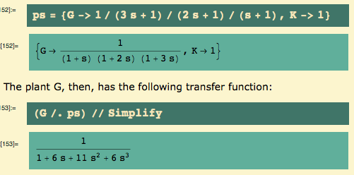
My plant is a 3rd-order transfer function… as usual, rules are a convenient way to specify things:

Control Theory – Example 2

Review

Let us recall Example 1. Carstens’ final solution was to take K =.032, so that the plant and the parameters were… and the open loop transfer function was:

The corner frequency (the breakpont) is still 4 rad/sec. Here’s the open-loop Bode plot.

Introduction to CAPM, the Capital Asset Pricing Model

introduction

It can be difficult to find a clear statement of what the Capital Asset Pricing Model (henceforth CAPM) is. I’m not trying to do much more than provide that. In particular, I did not find the wiki article to be useful, even after acquiring a couple of recent books on the subject.

I own six references:

• Sharpe, Wiliam F.; “Investments”, Prentice Hall, 1978; 0-13-504605-X.
• Reilly, Frank K.; “Investments”, CBS College Publishing (The Dryden Press), 1980; 0-03-056712-2.
• Gringold, Richard C and Kahn, Ronald N.; Active Portfolio Management, McGraw-Hil, 2000; 0-07-024882-6.
• Roman, Steven; Introduction to the Mathematics of Finance, Springer, 2004; 0-387-21364-3.
• Benninga, Simon; Financial Modeling, 3rd ed. MIT, 2008; 0-262-02628-7.
• Ruppert, David; Statistics and Data Analysis for Financial Engineering; Springer 2011; 978-1-4419-7786-1.

There is more than one version of the CAPM… Roman (p. 62) tells me that “The major factor that turns Markowitz portfolio theory into capital market theory is the inclusion of a riskfree asset in the model…. generally regarded as the contribution of William Sharpe, for which he won the Nobel Prize…. the theory is sometimes referred to as the Sharpe-Lintner-Mossin (SLM) capital asset pricing model.”

Then Benninga (p. 265) told me about “Black’s zero-beta CAPM… in which the role of the risk-free asset is played by a portfolio with a zero beta with respect to the particular envelope portfolio y.” (We’ll come back to this, briefly.)

Control Theory: Example 1 part 2

review: K = 1

Let us resume Example 1. We started with the following transfer function, for which I arbitrarily assumed K = 1 and that the given factor of 100 was part of the plant G. There are two poles at -4, and 0.

… which had the following open loop Bode plot

Control Theory – Example 1 P-only control

Introduction

Everyone under the sun seems to have their own way of organizing control theory. I may very well end up – I hope I end up – with a few different conceptual approaches for myself. But to begin with, I’m going to just start with examples, so that I’ve got a lot of material to try organizing. If you’re new to control theory, my beginning may seem rather chaotic. Sorry.

It is also my intention to stay with classical control theory for quite a while… I’ll move to state space after I’m comfortable with SISO – single input, single output – and the pre-state-space methodologies.

This first example does one positive thing: it illustrates the effect of proportional control.

It also does a few things that are not quite positive: that is, it raises a few questions. I’m more than a little glad it’s not perfectly straight-forward. Let me not keep secrets:

• Carstens’ first real design problem, later in the book, suggests that this solution is not an acceptable real-world design.
• Tuning rules such as Ziegler-Nichols, which require that the system be brought to the edge of instability, cannot be applied.
• Minimizing the obvious measures of error do not agree with his solution – although his looks pretty standard to me.

My point is not that his solution is incorrect, but that it’s sort of incomplete. It’s a student exercise. Let me rephrase that: I’m delighted to know if the solution to an exercise really is a real-world solution, regardless of whether it is or is not… just so I know which.

Let me start by grabbing a drawing from an earlier post.

Elementary Number Theory: the algebra of arithmetic functions

intro & Euler’s and…

I am going to look at several arithmetic functions, and we will see how Mathematica knows them. We will see the convolution product of arithmetic functions for dealing with particularly appropriate summations, the Möbius Inversion Formula, and we will see a conceptual basis for the Möbius function, which basis is part of a useful more conceptual way to deal with all these summations.

If you get bogged down along the way, skip to the final section entitled “Way too Easy!”

In fact, I have filed this post under “abstract algebra” because we’ll be doing just a little algebra to get a good grip on these functions. And yet that little will go a long, long way.

A function defined on the positive integers – which we would usually call a sequence! – is said to be multiplicative if

whenever m and n are relatively prime. (That is, whenever the greatest common divisor (GCD) of m and n is 1: we often use (m,n) for the GCD and write that condition as (m,n) = 1.) Be careful: we require that the function of a product be the product of the functions only when the integers are relatively prime, not for all pairs of integers m and n.

Control Theory – Simple Bode Plots

Minor edits 10/28/12: replaced “poles -1/tau” by “poles s = -1/tau” and at least one -1/tau by the absolute value of -1/tau.

We’re going to be looking at multiple Bode plots in one image. Despite everything I’ve shown you, it seems impossible to set both the color and the thickness. I believe this is a bug.

Here’s what happens if I try. (This happens to be a second-order system.)

So, we lost the color spec in the phase plots. I’ve tried a few other possibilities, but they don’t work either.