Example: Is it a transition matrix? Part 2

We had three matrices from Jolliffe, P, V, and Q. They were allegedly a set of principal components P, a varimax rotation V of P, and a quartimin “oblique rotation” Q.

I’ll remind you that when they say “oblique rotation” they mean a general change-of-basis. A rotation preserves an orthonormal basis; a rotation cannot transform an orthonormal basis to a non-orthonormal basis, and that’s what they mean — a transformation from an orthonormal basis to a non-orthonormal basis, or possibly a transformation from a merely orthogonal basis to a non-orthogonal one. In either case, the transformation cannot be a rotation.

(It isn’t that complicated! If you change the lengths of basis vectors, it isn’t a rotation; if you change the angles between the basis vectors, it isn’t a rotation.)

Anyway, we showed in Part 1 that V and Q spanned the same 4D subspace of .

Now, what about V and P? Let me recall them:

Example: Is it a transition matrix? Part 1

This example comes from PCA / FA (principal component analysis, factor analysis), namely from Jolliffe (see the bibliography). But it illustrates some very nice linear algebra.

More precisely, the source of this example is:
Yule, W., Berger, M., Butler, S., Newham, V. and Tizard, J. (1969). The WPPSL: An empirical evaluation with a British sample. Brit. J. Educ. Psychol., 39, 1-13.

I have not been able to find the original paper. There is a problem here, and I do not know whether the problem lies in the original paper or in Jolliffe’s version of it. If anyone out there can let me know, I’d be grateful. (I will present 3 matrices, taken from Jolliffe; my question is, does the original paper contain the same 3 matrices?)

Like the previous post on this topic, this one is self-contained. In fact, it has almost nothing to do with PCA, and everything to do with finding — or failing to find! — a transition matrix relating two matrices.

PCA / FA. Example 4 ! Davis, and almost everyone else

I would like to revisit the work we did in Davis (example 4). For one thing, I did a lot of calculations with that example, and despite the compare-and-contrast posts towards the end, I fear it may be difficult to sort out what I finally came to.

In addition, my notation has settled down a bit since then, and I would like to recast the work using my current notation.

The original (“raw”) data for example 4 was (p. 502, and columns are variables):

PCA / FA example 4: davis. Davis & Jolliffe.

What tools did jolliffe give us (that i could confirm)?

1. Z = X A, A orthogonal, X old data variables in columns
2. serious rounding
3. plot data wrt first two PCs
4. how many variables to keep?

but jolliffe would have used the correlation matrix. Before we do anything else, let’s get the correlation matrix for davis’ example. Recall the centered data X:

i compute its correlation matrix:

Now get an eigendecomposition of the correlation matrix; i called the eigenvalues and the eigenvector matrix A. Here’s A:

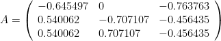
If we compute and get an identity matrix, then A is orthogonal. (it is.)

PCA / FA example 3: Jolliffe. analyzing the covariance matrix

we have seen what jolliffe did with a correlation matrix. now jolliffe presents the eigenstructure of the covariance matrix of his data, rather than of the correlation matrix. in order for us to confirm his work, he must give us some additional information: the standard deviations of each variable. (recall that he did not give us the data.)

we have to figure how to recover the covariance matrix c from the correlation matrix r, when for each and every ith variable we have its standard deviation .

it’s easy: multiply the (i,j) entry in the correlation matrix r by both and

the diagonal entries , which are 1, become variances , and each off-diagonal correlation becomes a covariance. maybe it would have been more recognizable if i’d written

which says that we get from covariances to correlations by dividing by two standard deviations.

here are the standard deviations he gives:

PCA / FA example 2: jolliffe. discussion 3: how many PCs to keep?

 

from jolliffe’s keeping only 4 eigenvectors, i understand that he’s interested in reducing the dimensionality of his data. in this case, he wants to replace the 8 original variables by some smaller number of new variables. that he has no data, only a correlation matrix, suggests that he’s interested in the definitions of the new variables, as opposed to the numerical values of them.

there are 4 ad hoc rules he will use on the example we’ve worked. he mentions a 5th which i want to try.

from the correlation matrix, we got the following eigenvalues.

we can compute the cumulative % variation. recall the eigenvalues as percentages…

now we want cumulative sums, rounded….

PCA / FA example 2: jolliffe. discussion 2: what might we have ended up with?

back to the table. here’s what jolliffe showed for the “principal components based on the correlation matrix…” with a subheading of “coefficients” over the columns of the eigenvectors.

under each column, he also showed “percentage of total variation explained”. those numbers were derived from the eigenvalues. we saw this with harman:

• we have standardized data;
• we find an orthogonal eigenvector matrix of the correlation matrix;
• which we use as a change-of-basis to get data wrt new variables;
• the variances of the new data are given by the eigenvalues of the correlation matrix.

the most important detail is that the eigenvalues are the variances of the new data if and only if the change-of-basis matrix is an orthogonal eigenvector matrix.

and that is what jolliffe has: the full eigenvector matrix P is orthogonal. OTOH, we don’t actually know that the data was standardized, but the derivation made it clear that if we want the transformed data to have variances = eigenvalues, then the original data needs to be standardized.

again, since jolliffe never uses data, we can’t very well transform it.

PCA / FA example 2: jolliffe. discussion 1: notation & vocabulary

Let’s do a little housekeeping. First off, Jolliffe ’s notation. Recall Harman’s:

where Z was the original data, variables in rows; A was a transition matrix, a weighted eigenvector matrix; and F was the new (transformed) variables wrt the basis specified by A.

In that case, each column of Z is an old vector equal to the application of A to the new vector in the corresponding column of F. This is fairly natural. If we let lower case z and f be corresponding columns of Z and F, then

We call A a transition matrix because it says that the old vectors z are the images under A of the new vectors f. Finally, the columns of A are the (old) components of the new basis vectors; the transpose of A is called the attitude matrix of the new basis vectors.

Let me emphasize that when I say “new data” I mean the data transformed using the transition matrix. Each observation is a vector, and that vector has components wrt the original basis and the new basis (the eigenvector basis). When I say “new data” I mean components wrt the new basis.

That was Harman.

PCA / FA example 2: jolliffe. correlation matrix

what we got from harman’s “factor analysis” was his only example of principal component analysis. now let’s see what jolliffe’s “principal component analysis” has for us.

i’m going to work one example, but he did it two ways, and i’ll confirm both sets of calculations.

first, he gives us a correlation matrix. i note that he says who gave him the data, but there is no other detail. don’t plan on ever finding the data behind this. here is the correlation matrix.

we know what to do: get the eigenstructure.