Color: from XYZ to spectrum

Introduction.

In this post, I will go from XYZ coordinates to a spectrum.

I have to ask: what would somebody do with this? Especially, what would they do that couldn’t have been done using the XYZ tristimulus values directly? I don’t know – but let’s just solve the problem. I do not yet always have a satisfactory solution, and I will illustrate both satisfactory and unsatisfactory solutions.

Yes, we have done this before – but not as our primary purpose, but rather as part of another computation. It is worthwhile to tackle this specific problem, because there is one subtlety.

In general terms, the solution is simple: the XYZ tri-stimulus values are proportional to the components (with respect to the dual basis) of a (fundamental) spectrum. Find the dual basis, then get the linear combination defined by those components.

I am going to use the CIE 1931 color matching functions. I will show the calculations explicitly for 20 nm intervals, but I will show graphs for both the 20 nm intervals and for 5 nm intervals.

A nice example. (A satisfactory solution.)

Here is a swatch of color.

The digital color meter on my computer says that this swatch has…

{X, Y, Z} = {67.422, 82.956, 35.834}

and RGB = {66.3, 100.0, 54.1} . (I chose it off the color wheel, and Mathematica translated my click into an RGB specification, namely RGBColor[0.663767, 1, 0.541878]. So the RGB reported by the digital color meter matches what I put in – which was selected off the HSB color wheel by sight (not by value).)

Incidentally, on my Mac, the calculator in the ColorSync utility confirms these two triples – just input XYZ as “perceptual”, and read off the RGB. Oh, remember to set the device to “LCD”, because the utility opens with “generic RGB”. You may have counted that I am using two pieces of software, the DigitalColor Meter and ColorSync.

So let’s go get a spectrum for that swatch.

We have learned that the XYZ tri-stimulus values are proportional to the components of a fundamental spectrum with respect to the basis E dual to the color matching functions in the matrix A.

That proportionality constant has always been computed by applying the second row of A’ to the spectrum of the illuminant. It appears, therefore, that we will need to choose an illuminant.

We do not need to, and we probably shouldn’t – but we can, and I will choose one the first time I do this calculation.

Okay, we need a matrix A and the dual basis E. For graphing, it will be convenient to have a list of wavelengths.

What range of wavelengths? Well, the color matching functions I have (at 5 nm intervals) are defined over 380 – 780 nm. That is smaller than the range over which illuminants are defined, so I might as well choose the entire range of the color matching functions. It is the smaller, hence the limiting, range.

Here are the wavelengths…

{380, 400, 420, 440, 460, 480, 500, 520, 540, 560,
580, 600, 620, 640, 660, 680, 700, 720, 740, 760, 780}

Let me choose a common standard illuminant, D65. Here it is…

{50., 82.8, 93.4, 104.9, 117.8, 115.9, 109.4, 104.8,
104.4, 100., 95.8, 90., 87.7, 83.7, 80.2, 78.3, 71.6,
61.6, 75.1, 46.4, 63.4}

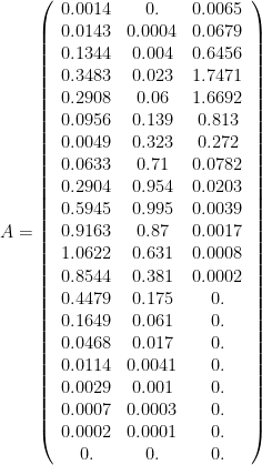
Here is my A matrix, from the CIE 1931 XYZ (xyz bar) tables at 20 nm intervals.

Now we can compute the scaling factor: apply the transpose A’ to d65, and take the middle number as the scaling – or, instead, just apply the middle row of A’ to d65…

s1 = 529.642

then we multiply our XYZ by that scale, to get components wrt the dual basis E…

c1 = s1 {X, X, Z} = {35709.5, 43937., 18979.2}.

Now get the dual basis. As usual, we define the dual basis by its action on the columns of A…

E’A = I,

where I is a 3×3 identity matrix. Then we write the utterly impossible

,

because it reminds us of the true formula which uses the pseudo-inverse:

.

Thus I compute E’, but display the transpose (because it fits on the screen)…

From the components and the basis vectors (rows of E’), I compute the fundamental as a linear combination…

f1 = c1.ET = {13.7722, 147.654, 1404.24, 3909.35, 4082.99, 3075.15,
3862.37, 7568.38, 10233.7, 10959.3, 10011.9, 7694.61, 4877.98,
2300.89, 811.6, 227.105, 54.8956, 13.5196, 3.87036, 1.25375, 0.}

It is a perfectly nice spectrum, always non-negative.

Let’s look at it:

Here’s a picture from my (unpublished) computations at 5 nm intervals.

Let’s check the computation. From that spectrum, we recover the components wrt E by applying A’…

{35709.5, 43937., 18979.2}

then divide by the scale…

{67.422, 82.956, 35.834}

which is exactly the given XYZ…

{X, Y, Z} = {67.422, 82.956, 35.834}

Now hold up a minute.

How did we check that answer? We got the components of that spectrum with respect to the E basis – but that just used A’. Oh, then we divided by the scale factor, which came from D65.

Not really. I didn’t recompute the scale factor… I just used the same one as before. And that’s the point. If we want to check the answer, by reversing the calculations, we have to know what scale factor was used to get from XYZ to the components.

It doesn’t matter what that scale factor is or where it came from, it just has to be the same one when we check the answer as when we combined the basis vectors.

We could have used 1 or 100, or pi, in order to get from XYZ to the components. If someone aks me for the illuminant, I’m going to answer the question they should have asked in this case, and tell them the scale factor (which may, but need not, have come from an illuminant).

In fact, now that I look at the scale on the graph, that spectrum is pretty intense in any customary units. Maybe I should have used 1 instead of about 500.

If you’re uncomfortable with using an arbitrary scale factor, and want to specify an illuminant, but D65 seems too special, consider using an equal-energy illuminant instead of D65. It doesn’t matter, as far as I can see.

A not-so-nice example. (An unsatisfactory solution.)

Here is another set of XYZ…

{X, Y, Z} = {30.64, 19.812, 8.203}

The ColorSync utility tells me that on my monitor, those are RGB…

(and DigitalColor Meter then confirms that this RGB spec has the given XYZ).

That is, in this case I had a set of XYZ tri-stimulus values at my fingertips. The ColorSync utility lets me find the RGB which my monitor believes is equivalent, so I know what to feed Mathematica for that disk. This achieves one outstanding goal: given XYZ, I can find out what color it represents on my monitor. (That’s a nonlinear calculation, and so far, I’m letting the computer do it implicitly.)

In the first case, I had picked a color, gotten the RGB first, and then asked for the tri-stimulus values from the image. When I go the other way, I first have to let the computer calculate RGB from XYZ – and then I can confirm the two sets of numbers from the image.

Anyway….

For this case, let’s just set the scale factor equal to 1. This means that our XYZ values are themselves the components with respect to the three E basis vectors.

We compute the fundamental as a linear combination of the basis vectors, and get…

f4 = {X, Y, Z}.ET = {0.0111122, 0.111361, 1.04104, 2.61278, 1.92543,
0.116112, -1.05328, -1.39481, 0.440321, 3.67812, 7.57807, 9.86993, 8.30289,
4.42371, 1.63849, 0.465915, 0.11361, 0.0290242, 0.00683746, 0.00191253, 0.}

Some negative numbers. Let’s look at it.

Again, here’s the corresponding picture from my (unpublished) computations at 5 nm intervals.

I assure you, this spectrum being negative around 500 nm has nothing to do with my choice of scaling factor. The scaling factor only affects the vertical scale, not the origin; it doesn’t translate the curve.

Are these negative values OK?

I don’t know. Why did we want this spectrum? What are we going to do with it? And, as I asked before, could we have done it all with just the XYZ values?

As it happens, however, I know a way to fix this, in this case…. We can eliminate the negative values. I know a residual which I can add to it to this spectrum, so that the sum will be everywhere positive – and since I’m adding a residual, it has no effect on the XYZ values.

Truth to tell, I know two or three residuals which will make the negatives become positive. One of them is the residual from an equal-energy illuminant.

Let’s see that.

Now the quickest way to get a residual is to subtract a fundamental from a spectrum… and the quickest way to get a fundamental, in general, is to apply a projection operator to a spectrum.

Been there, done that. We recall that we can construct a projection operator onto the 3D color-fundamental subspace as follows. Let u,w,v be the Singular Value Decomposition of A’:

A’ = u w v’.

Let v1 be the first 3 columns of v. Then the 3 columns of v1 are an orthonormal basis for the pre-image of the range of A’ (the color-fundamental subspace) , and the matrix

P = v1 v1′

is a projection operator onto the span of v1 (again, the color-fundamental subspace).

I ask for the SVD:

{u,w,v}=SingularValueDecomposition[AT];

I get v1 as the first 3 columns of v:

Then I define

P = v1 v1′.

Now, p is 21×21, so I’m not going to display it… but for checking purposes, here are its first row…

second-to-last row (the last row is identically zero)…

and its first column…

Next, here’s an equal-energy spectrum…

ee=ConstantArray[100,21]
= {100, 100, 100, 100, 100, 100, 100, 100, 100, 100, 100,
100, 100, 100, 100, 100, 100, 100, 100, 100, 100}

Here’s its fundamental… P.ee =

{0.470329, 4.93178, 46.8236, 126.976, 122.475, 67.1406, 46.2149,
73.0368, 104.313, 123.805, 129.975, 116.133, 81.8326, 40.6347,
14.6472, 4.12848, 1.00191, 0.250948, 0.0659255, 0.0201401, 0.}

Here is its residual… re = ee-P.ee =

{99.5297, 95.0682, 53.1764, -26.9757, -22.4752, 32.8594, 53.7851,
26.9632, -4.31253, -23.8048, -29.9753, -16.133, 18.1674, 59.3653,
85.3528, 95.8715, 98.9981, 99.7491, 99.9341, 99.9799, 100.}

And here’s what the residual looks like. Note that the scale is much smaller than for our fundamental spectrum.

Again, here’s the corresponding picture from my (unpublished) computations at 5 nm intervals.

Now let’s see if I can add some of that residual to the fundamental, and end up with something nice.

Playing around, I discover that this works: f4 + 8re/100 =

{7.97349, 7.71682, 5.29515, 0.454721, 0.127414, 2.74487, 3.24952,
0.762244, 0.0953185, 1.77374, 5.18005, 8.57929, 9.75627, 9.17293,
8.46672, 8.13564, 8.03346, 8.00895, 8.00156, 8.0003, 8.}

And the result looks like this:

Again, here’s the corresponding picture from my (unpublished) computations at 5 nm intervals.

(Blue is the original, the fundamental, sometimes negative. Black is the result of adding that particular residual.)

So, I grabbed the residual of an equal-energy illumninant, and added enough of it to make the sum positive everywhere. It had a pretty significant impact on the spectrum – but the XYZ values are unchanged, because I added a residual.

The residual of D65 would also work.

But the residual of illuminant C does not work. (I can get to a point where two values are negative, but changing things a little moves them in opposite directions. That won’t work.)

So it appears that I just lucked out. A multiple of the residual from either the D65 or the equal-energy illuminant can be added to this spectrum to give something which is everywhere positive. But not every residual of an illuminant will work.

Well, I didn’t really think it would. I just thought illuminants were a convenient source of real residuals.

(No, I don’t know how to tell ahead of time if a given {X, Y, Z} will have a fundamental which goes negative. Nor do I mean to assert that “correcting” that negativity is the only reason we might want to add a residual.)

I don’t yet know how to solve this problem of designing residuals to order, but I have an idea or two. I’ll keep you posted.