Let us now recall what we saw harman do. Does he have anything to add to what we saw davis do? if we’re building a toolbox for PCA / FA, we need to see if harman gave us any additional tools.
here’s what harman did or got us to do:
- a plot of old variables in terms of the first two new ones
- redistribute the variance of the original variables
- his model, written Z = A F, was (old data, variables in rows) = (some eigenvector matrix) x (new data)
We should remind ourselves, however, that harman used an eigendecomposition of the correlation matrix; and the eigenvectors of the correlation matrix are not linearly related to the eigenvectors of the covariance matrix (or, equivalently, of  .) having said that, i’m going to go ahead and apply harman’s tools to the davis results. i will work from the correlation matrix when we get to jolliffe.
What exactly was that graph of harman’s? he took the first two columns of the weighted eigenvector matrix, then plotted each row as a point. He had 5 original variables. His plot

shows that the old 1st and 3rd variables, for example, are defined very similarly in terms of the first two new variables. let me emphasize that this is a description of defining variables, not a display of the resulting data. Simple counting can help with the distinction, e.g. 3 variables but 4 observations.
Read the rest of this entry »


 .
. .
. .
. .
. instead of the SVD.

 and the eigenvector matrix A. Here’s A:
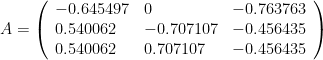
 and get an identity matrix, then A is orthogonal. (it is.)
 for the SVD of X.)

 is very well behaved. Its two columns are orthogonal to each other:
 are the components wrt the reciprocal basis, we ought to find the components wrt the


 is the new data wrt the orthogonal eigenvector matrix; and i hope i’ve said that the R-mode scores
  are not the new data wrt the weighted eigenvector matrix


 ; but what if X doesn’t have row-centered data?)
 and
and 

