Color: from spectrum to tristimulus

Introduction

Edit 30 Oct 2009:
This is the first post about an example on p. 160 of Wyszecki & Stiles (see the bibliography).

and find another edit about the components wrt the dual basis.
End edit.

As always, if my chatter is confusing, just start following the examples.

In a sense, what I am about to do now is one of the most important color calculations I will show you.

How do we get from a spectrum to tristimulus values?

I am going to get from a spectrum to XYZ values, and then to xyz values. Recall that XYZ come from xyz bar tables, which in turn come from rbar, gbar, bbar tables by a change of basis. Then xyz values come from XYZ by making the sum = 1.

For more about the CIE, see the previous post.

The question before us is to get from a spectrum to XYZ (and then to xyz).

What we are talking about is the perception of color, rather than the reproduction. Sort of. We wil use “the standard observer” rather than my eyes or your eyes, but we are going to translate an arbitrary spectrum into 3 scalar values, which can then be transformed to some RGB values in a color space. But not in this post.

This example comes from w&s (Wyszecki & Stiles, in the bibliography), page 160. Believe it or not, I am going to work it four ways — but I will give you the full details for only two of them, pictures for all four of them.

The original problem uses data at 10 nm intervals, and it uses the 1964 CIE. Working this example as they did showed me that there were 3 typos in their solution.

First, however, I will work the problem using the data at 20 nm intervals, with the 1964 CIE. This will show you explicitly how the calculations proceed. At 20 nm intervals, I can display the data itself.

Second, I will work the original problem as they posed it. I will not get their answers, so I will also show you their typos.

Third and fourth, I will again work the problem at both 10 nm and 20 nm intervals, but using the 1931 CIE. As will be my ongoing custom, I will show you all the numbers only for the 20 nm case. Ultimately, what choice we make isn’t going to matter a lot. And that’s worth knowing.

We are given a reflectance spectrum for a plastic object illuminated by daylight. In fact, we will use “standard illuminant D65” for “daylight”. The “reflectance spectrum” is the reflection from a perfectly uniform — perfectly equal energy — illuminant.

Let me say that another way. We are going to assume that the object is illuminated by one spectrum (“daylight” D65) and that the reflected spectrum which we perceive is the combination of the D65 spectrum and the so-called reflectance spectrum of the object.

The reflectance spectrum is a property of the object; by combining it with any arbitrary illumination spectrum, we get the reflected spectrum.

We are asked, in the given example, to find the XYZ tristimulus values, and the xy chromaticity coordinates, using the 1964 CIE color matching functions. That is, we will use the 1964 xyzbar tables.

(I didn’t plan to show this to you, but prudence dictated that I at least work it out. When it turned out that they had slightly wrong answers… well, I have to show it to you.)

Here’s what we will do. We will find the reflected spectrum, i.e. what is reflected from the object illuminated by D65 rather than by an equal energy illumninant. Then we will apply the xyzbar color matching functions to the reflected spectrum to get XYZ tristimulus values. Then we will get the normalized xyz values.

For more about the color matching functions, our matrices A for each problem, see the first Cohen post, and the second Cohen post.

CIE 1964 at 20 nm

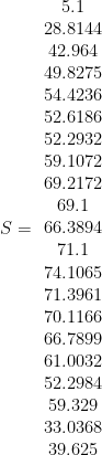
Here is the reflectance spectrum , from 380 to 780 at 20 nm intervals. As will be my custom, I am taking a subset of their values — I am not averaging the numbers. That is, their example provides data every 10 nm, but I am using half of that given data. For one thing, as I said, that gives us matrices of manageable size.

Here’s a picture of that reflectance spectrum:

A word about scaling. It is appropriate that the reflectance spectrum be less than, or on the order of magnitude of, 1. At any given frequency, the amount reflected can range from significantly less to significantly more (since light absorbed at one frequency can be emitted at another) than the incident spectrum — but we dont want to be multiplying by a hundred. That would be bad.

Here is the D65 spectrum, from 380 to 780 nm at 20 nm intervals:

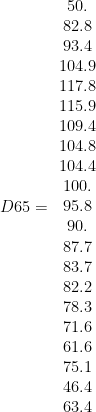
Another word about scaling. The D65 spectrum ranges from 50 to more than 100. I have no idea what units it is measured in — but the reflected spectrum will be in the same units, whatever they are.

Here is a picture of that illumninant spectrum:

As I said, the scale is 100 times that of the reflectance spectrum. This doesn’t matter for the computations. If, however, I want to show both of these on the same axes, I will need to scale these values — but for the graph only, not for the computations.

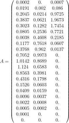
Here are the 1964 xyzbar tables from 380 to 780 nm, at 20 nm intervals. This is the A matrix for this problem.

And here is a picture of the color matching functions:

Those are our ingredients: the reflectance spectrum, the illiminant spectrum, and the color matching functions.

Now, let’s get the reflected spectrum. We multiply the values pointwise… i.e. at every wavelength, what is actually reflected is the product of the reflectance spectrum and the illuminant spectrum.

(Perhaps I should be calling this the perceived spectrum, since it is what our standard observer is seeing. I should not call it the incident spectrum, because that would be a sensible alternative to “the illimination spectrum”, in this case D65. Incident illumination on an object gives us a reflected spectrum, which our standard observer perceives.)

The result of multiplying the reflectance spectrum and the illuminant spectrum D65 is

and the 3 spectra look like this (after I divide the D65 and S by 100, otherwise the reflectance spectrum is effectively the x-axis):

Let’s be clear: the reflectance spectrum is in green, the illuminant spectrum is in blue, and the product, at each wavelength, is the reflected spectrum, in black.

Before we deal with the reflected spectrum, however, I want to deal with the illumination itself. If we apply the color functions to the D65 spectrum, that is we compute

,

we get

{554.645, 582.565, 631.147}.

Are those our tristimulus values? No way. These numbers depend on the scale of the spectrum, and the number of components of the vectors. Somehow we have to normalize them, and we will do that for the total energy received.

As an aside, which I will try to remember to repeat in subsequent posts…. We have spectra and color-matching functions which live in vector spaces. The result of applying color matching functions to spectra is a set of 3 scalars, i.e. 3 real numbers. But our vector spaces are not bounded spaces, so those 3 numbers are not, in principle, bounded. They are simply the components of a spectrum wrt a basis. Edit: oops. Careful! They are components of the fundamental of the spectrum. End edit. OTOH, we have color spaces, such as RGB, in which the RGB values are bounded (whether between 0 and 1, or 0 and 100, or 0 and 255, they are limited).

We need to move from the unbounded results of vector operators to the bounded values of color spaces.

But how do we do that?

Well. Recall that ybar, the second column of A, is the photopic response (the total response of the cones) of the standard observer. This is incredibly useful: the second column of AT tells us the total energy perceived. If we were doing calculus, we would compute the areas under all three curves. But we’re doing linear algebra, and the appropriate number is the middle one.

We get XYZ values for the illumnination perceived by the observer by dividing those 3 numbers by the middle number, 582.565:

XYZ = {0.952075, 1., 1.08339}.

Let’s keep going with this. How do we get xyz coordinates from XYZ?

Normalize the sum of the XYZ to 1. The sum is 3.03547 … so we get that x,y,z are

xyz = {0.31365, 0.329438, 0.356911}.

Since all three values are close to 1/3, this is a plausible number for illumination.

Now we can do the same thing with the reflected spectrum. That is, we apply the matrix to the reflected spectrum S:

{386.796, 381.417, 293.87}.

We are not going to divide by this middle number — this is the reflected spectrum, not the illimination spectrum. We need to divide by the same number as before, i.e. by the photopic response to the illumination, not the photopic response to the reflection. That number was 582.565, and now we divide our 3 values by that to get X,Y,Z…

XYZ = {0.663953, 0.654719, 0.504441}.

And, as before, we compute xyz values, too: we normalze the XYZ so that their sum is 1. Since the sum is 1.82311 … we get

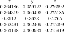
xyz = {0.364186,0.359122,0.276692}.

This isn’t all that far from the illuminant.

Those dots are the outline of the 1964 chromaticity diagram. I got it the same way as the 1931, just with different data. Get the xyz tables — the ones where the rows add up to 1 — and just plot y versus x.

The red, green, and blue dots show the pure primaries for the 1964 standard. The white dot is (x,y) for D65, and the yellow dot is (x,y) for the reflected sprectrum. (Oh, I don’t think the reflection is yellow, but it’s rather closer to the light source than to much else.)

CIE 1964 at 10 nm

Now let me show you the pictures, and the answers, for 10 nm intervals. In fact, let me juxtapose the new pictures (on the right) with the old (on the left):

Here are the old and new reflectance spectra:

Here are the D65 spectra:

And here are the color matching functions (xyzbar tables) from 380 to 780 nm The data on the right is the A matrix for this problem.

We have the same ingredients: the reflectance spectrum, the illiminant spectrum, and the color matching functions.

Now, let’s get the reflected spectrum. We multiply the values pointwise… i.e. at every wavelength, what is actually reflected is the product of the reflectance spectrum and the illuminant spectrum.

The result of multiplying and D65 together looks like this (after I divide the D65 and S by 100, otherwise the reflectance spectrum is effectively the x-axis):

As before, the reflectance spectrum is in green, the illuminant spectrum is in blue, and the product, at each wavelength, is the reflected spectrum, in black.

First, we apply the color functions to the D65 spectrum, that is we compute

,

and we get

{1102.11, 1162.02, 1247.78}.

Here we see quite clearly that these numbers depend on the scale of the spectrum and the number of values: they are about double what the previous values were. Oh, of course: our vectors are twice as long. (Even though the XYZ and xyz values will be comparable, these initial 3 values will not always be comparable. As I said, they depend on the dimension of our spectra and on the scaling of the illuminant spectrum.)

Once again, we need to scale those numbers, dividing each of them by the middle number, which is the total perceived illumination.

So we get XYZ values for the illumninant by dividing those 3 numbers by the middle number, 1162.02:

XYZ = {0.948445, 1., 1.0738}.

How do we get xy coordinates? Normalize the sum to 1. The sum is 3.02225 … so we get

xyz = {0.313821, 0.330879, 0.3553}.

As before, this is a plausible number for illumination.

Now we do the same thing with the reflected spectrum. That is, we apply the matrix to the reflected spectrum S:

{769.263, 761.189, 581.056}.

Once again, we divide by the same number as before, i.e. by the photopic response to the illumination, not to the reflection. (That number was 1162.02.)

Now we divide our 3 values by that to get X,Y,Z…

XYZ = {0.662005, 0.655057, 0.50004}.

And, as before, we compute xy values, too: we normalze the XYZ so that their sum is 1. Since the sum is 1.8171 … we get

xyz = {0.364319, 0.360495, 0.275185}.

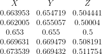
You can’t tell much from these two pictures; the final picture in this post will plot (almost) all of the xy answers. The numbers using 20 nm intervals were not much different: for the XYZ values of the reflected spectrum, we had:

XYZ = {0.663953, 0.654719, 0.504441}.

The corresponding answers using 10 nm intervals were:

XYZ = {0.662005, 0.655057, 0.50004}.

Pretty darn close. 10 nm or 20 nm, both using CIE 1964, not a whole lot of difference.

Now, what were their answers? They got sums of

{758.6, 760.8, 580.8}

… while I had

{769.263, 761.189, 581.056}.

We do not agree. What’s going on? I found that there is a problem in their work at 640 nm.

For a wavelength of 640 nm, we agree on the values of all the ingredients. We agree that the reflectance spectrum value is 0.853 … the D65 illuminant spectrum value is 83.7 … the values of that row of A are {0.4316, 0.1798, 0.}.

The pointwise products of these numbers are…

{30.8146, 12.837, 0.}

but what they show is

30.2 12.6 0.

Two typos. I have no idea why. And they appear to be the only typos pertaining to individual wavelengths. Of course, it is possible that the error is in the reflectance spectrum instead, but I have no other data-source to compare that to. In any event, it is clear that their entries (30.2 and 12.6) are not in fact the product of the inputs they show.

There’s another problem. I pasted the column that leads to the X-column-sum into a spreadsheet and computed the sum. For the data they have shown, the first sum is really 768.6 rather than 758.6 . That’s the third typo.

(In addition, they round off at each wavelength, before adding the columns: this leads to some round-off error. That’s why we differ on the sum that leads to Z; no typos there, they just rounded before adding.)

But, where they show X,Y,Z as (change of scale, decimals versus percentages; ignore it) …

XYZ = {65.3, 65.5, 50.}

the correct answers are

XYZ = {66.2005, 65.5057, 50.004}

and even using 20 nm intervals instead of 10, I got

XYZ = {66.3953, 65.4719, 50.4441}.

For x,y, they show

xy = {0.3612, 0.3623}

but correct (at 10 nm) is

xy = {0.364319, 0.360495}.

Just working at half the resolution (20 nm), I got

xy = {0.364186, 0.359122}.

I daresay their mistakes are worse than my cutting the resolution in half.

CIE 1931 10 nm

To switch from 1964 at 10 nm to 1931 at 10 nm requires only that I change the A matrix. (I have everything else in memory at 10 nm intervals. The reflectance, reflected, and D65 spectra do not change.)

Let me show 1931 on the right, for comparison with the 1964 color matching functions on the left. Note that the vertical scales are different.

Although they have not changed, I show again the reflectance spectrum and the illuminant spectrum for this case:

Go ahead, curse me out. After showing different cases side-by-side, I have just switched and shown side-by-side graphs for two different things for one and the same case.

Those are our ingredients: the reflectance spectrum, the illiminant spectrum, and the color matching functions. Only the color functions have changed, from 1964 to 1931.

Now, the pointwise product of the illuminant and reflectance spectra will be exactly the same reflected spectrum.

Let’s be clear: the reflectance spectrum is in green, the illumninant spectrum is in blue, and the product, at each wavelength, is the reflected spectrum — in black.

As before, we apply the color matching functions to the D65 spectrum, that is we compute

,

getting

{1004.46, 1056.89, 1150.02}.

These numbers are comparable to the previous case: we are using vectors of the same dimension.

Once again, we need to scale those numbers, dividing each of them by the middle number, which is the total perceived illumination.

So we get XYZ values or the illumninant by dividing those 3 numbers by the middle number:

XYZ = {0.950398, 1., 1.08812}.

To get xy coordinates, we normalize the sum to 1. The sum is 3.03852 … so we get

xyz = {0.312783, 0.329108, 0.358109}.

Now we do the same thing with the reflected spectrum. That is, we apply the matrix to the reflected spectrum S:

{707.724, 707.564, 537.101}.

Once again, we divide by the same number as before, i.e. by the photopic response to the illumination, not to the reflection. That number was 1056.89 .

So we divide our 3 values by that to get X,Y,Z…

XYZ = {0.669631, 0.669479, 0.508191}.

And, as before, we compute xy values, too: we normalze the XYZ so that their sum is 1. Since the sum is 1.8473 … we get xyz as

xyz = {0.362491, 0.362409, 0.275099}.

Again, this isn’t all that far from the illuminant. We’re getting very similar answers.

The CIE boundaries look pretty similar, but the triangles — the gamut of the 3 primaries — are different. And recall that the line x + y = 1 is tangent to the right-side boundary; furthermore, for the 1931 CIE, one side of the triangle is very, very close to the tangent line.

CIE 1931 20 nm

Having shown you pictures with the 1931 CIE and 10 nm intervals, let me close by showing you the numerical data, as well as pictures, for the 1931 CIE 20 nm solution.

To switch to 20 nm intervals, I need to rebuild the color matching functions. Here’s the data:

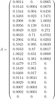
and here are the graphs (20 nm and 10 nm side by side):

I need to restore the reflectance spectrum and the illuminant spectrum. As you recall, they were

and

The reflected spectrum was the pointwise product of those, namely

Those are our ingredients: the reflectance spectrum, the illuminant spectrum, and the color matching functions. Only the color functions have changed, from 1964 to 1931.

The product of illumninant spectrum and reflectance spectrum is the same as shown before for 20 nm intervals:

As before, the reflectance spectrum is in green, the illumninant spectrum is in blue, and the product, at each wavelength, is the reflected spectrum — in black.

As before, we apply the color matching functions to the D65 spectrum, that is we compute

,

getting

{506.693, 529.764, 581.089}.

These numbers are smaller than the previous case: we are using vectors of half the dimension.

Once again, we need to scale those numbers, dividing each of them by their middle number, which is the total perceived illumination.

So we get XYZ values or the illumninant by dividing those 3 numbers by the middle number, getting:

XYZ = {0.956451, 1., 1.09688}.

We get xy coordinates by normalizing the sum to 1. The sum is 3.05333 … so we get

xyz = {0.313248, 0.327511, 0.359241}.

Now we do the same thing with the reflected spectrum. That is, we apply the matrix to the reflected spectrum S, getting:

{356.817,354.641,271.109}.

Once again, we divide by the same number as before, i.e. by the photopic response to the illumination, not to the reflection. That number was 529.764, so we get XYZ are

XYZ = {0.673539, 0.669432, 0.511754}.

And, as before, we normalze the XYZ so that their sum is 1. Since the sum is 1.85472 … we get

xyz = {0.363148 ,0.360933, 0.275919}.

OK, let’s compare.

Here are the unscaled sums (including their incorrect answers). Reading down, these are my 1964 at 20, then at 10, their answers, my 1931 at 10, then at 20.

and the XYZ values scaled by the photopic response…

and the xyz values

There’s not a whole lot of difference there, whether we use 1931 or 1964, or 10 nm or 20 nm, or make a few mistakes!

To look at it, here are my 4 computed xy, “white points”, for the illuminant, and the 5 xy points for the reflections.

(I didn’t grab their white point — the x,y coordinates — for D65, so only my 4 computed values are shown.)

The most important single computation in all this was to scale the values by the middle sum, i.e. by the total energy perceived by the observer. To be specific, we applied the ybar function to the illuminant spectrum.

I know, it looks just like the dot product of two vectors. But Cohen taught us that the color functions are really linear functionals. We want to visualize that computation as the matrix product of a row (the ybar) and a column (the D65 spectrum).

Of course, only such a trick as that division by the middle number could distract us from the marvelous computation of 3 numbers in the first place. We get from a spectrum to 3 scalars by applying 3 color matching functions (the transpose of our A matrix) to the reflected spectrum, which is also the spectrum incident on the eyes of the standard observer.

The first 3 numbers we get are, as we saw before and will see again, the (potentially unbounded) components of the incident spectrum wrt the dual basis spectra. The second set of 3 numbers are tristimulus values in XYZ space. The third set of numbers were xyz coordinates for the chromaticity chart.

The first 3 numbers depend on the dimensionality of our spectra, how many samples we have. In fact, we compute two such sets: one for the illuminant and one for the reflection. The middle number of the 3 for the illuminant sets the scale for white = (1,1,1).

The second set, XYZ, is found by dividing the first 3 numbers by that middle number. That is true whether we have XYZ for the illuminant or for the reflection: divide either by the total energy of the illuminant.

The third set, xyz, is found by dividing the XYZ numbers by their sum — instead of by their middle, or anybody’s middle.

I must emphasize that we have seen 4 different choices for the A matrix, and those were all “xyz bar” values! “The” A matrix is hardly unique.

More to come. You better believe it.