Introduction
I will close my discussion of the (Mathematica®) properties of a regression with “selection criteria” or “measures of improvement”: how do we select the “best” regression?
While I will do a couple of calculations, most numerical work with these criteria will wait until the next regression post.
Mathematica provides 4 such measures: R Squared, Adjusted R Squared, the Akaike Information Criterion (AIC), and the Bayesian Information Criterion (BIC).
In addition, I know almost a dozen more, and I’ll show them to you.
Almost all of them use the error sum of squares ESS; the R Squared and the Adjusted R Squared also use the total sum of squares TSS:


and the numbers n and k…
n = number of observations
k = number of parameters (
R Squared and Adjusted R Squared
The R Squared is
R2 = 1 – ESS / TSS.
It is 1 if and only if ESS = 0, i.e. there are no errors… y = yhat… the fit is exact at every data point.
This may or may not be a good thing.
In addition, there is a crucial fact pertaining to the use of R Squared as a measure of improvement: if we add a variable to a regession, the R Squared cannot decrease. It doesn’t have to go up, but it cannot get smaller.
In other words, as a measure of improvement, R Squared says we’re never worse off adding a variable. It can never recommend against adding a variable (until we have k > n, at which point the regression will fail, because X’X cannot be inverted).
The Adjusted R Squared is
Adjusted R Squared = 1 – (ESS/n-k) / (TSS/n-1).
As I have said before, it can be interpreted as subtracting the ratio of two estimates of variance. Like the R Squared, it is 1 if there are no errors.
But if we add a variable whose t-statistic is less than 1 (in absolute value), then the Adjusted R Squared will decrease. It does balance complexity (more variables in the model) against smaller total squared error.
In contrast to every other measure we will see here, we want its maximum rather than its minimum.
The AIC and BIC
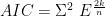
The AIC, as Mathematica uses it, appears to be defined as
![n\ Log[\frac{ESS}{n}]+2(k+1)+n Log[2Pi]+n](https://s0.wp.com/latex.php?latex=n%5C+Log%5B%5Cfrac%7BESS%7D%7Bn%7D%5D%2B2%28k%2B1%29%2Bn+Log%5B2Pi%5D%2Bn&bg=ffffff&fg=000000&s=0&c=20201002)
It is more than convenient to use rules at this point, so that I can write symbolic equations involving n, k, and ESS without having Mathematica use the numerical values of them.
Let me clear the numerical values… set some rules… then ask for the AIC for the regression (our main one, the Hald data with X1, X2, and X4, which can be found here)… and finally compute it directly using the equation…

Good. The regression AIC agrees with that equation.
(By the way, the //.ps said keep applying the rules until nothing changed. You might have noticed that the rule for ESS was incomplete: it used the numerical value of s^2, but symbolic n and k. That is, while it replaced n and k by numbers, it also introduced n-k. It took another pass to replace n-k by a number.)
The BIC from Mathematica is very similar; it has (k+1) log n where the AIC has 2 (k+1):
![n\ Log[\frac{ESS}{n}]+(k+1) Log[n]+n Log[2Pi]+n](https://s0.wp.com/latex.php?latex=n%5C+Log%5B%5Cfrac%7BESS%7D%7Bn%7D%5D%2B%28k%2B1%29+Log%5Bn%5D%2Bn+Log%5B2Pi%5D%2Bn&bg=ffffff&fg=000000&s=0&c=20201002)
Let me confirm that that equation agrees with the regression:

As usual, I am happy to see that I know exactly what Mathematica did for me.
Additional Selection Criteria
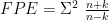
I was thrilled to find a table of selection criteria in Ramanathan (see bibliography page). Let me offer you the same thrill, augmented by another set of measures (all those subscripted with c or u, but also including the unsubscripted FPE) found in McQuarrie & Tsai’s “Regression and Time Series Model Selection”, ISBN 981 02 3242 X.
Let


You may recognize those as the minimum variance estimate and maximum likelihood estimate of the error variance 

Then we may define the following:


We see that every one of them chooses between 
They are all of the form: either
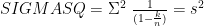
SIGMASQ is far and away the simplest. In fact, it is equivalent to the Adjusted R Squared: one increases if and only if the other decreases. It appears that Ramanathan wrote SIGMASQ in terms of
This shows us that we could write all of these in terms of 

Let me emphasize that the point of these measures is to assess the combined changes in ESS and k for a set of regressions having the same number of observations (and based on a common set of variables). The point is that n is a constant, while ESS (and
Why don’t we just stay with the Adjusted R Squared? I tell you, again, without proof, that adding a variable to a regression will raise the Agjusted R Squared if and only if the t-statistic for that variable is greater than 1 (in absolute value). But we might argue that the variable isn’t really significant unless its t-statistic is greater than about 2, which means that the Adjusted R Squared can improve when the regression, in one sense, does not.
We fear, then, that the Adjusted R Squared will “over fit” an equation, and we want something more conservative.
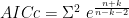
They tell me that the AIC is not sufficiently conservative, so we try other things.
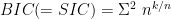
Oh, many of these are named for their inventors. On the other hand, FPE stands for Final Prediction Error – it was invented by Akaike, before he invented the AIC. He also invented the BIC, named the Bayesian Information Criterion. It is also known as the SIC, for Schwarz, who invented it independently. In fact, Ramanathan calls it SCHWARZ, and McQuarrie & Tsai call it SIC, while Mathematica calls it BIC.
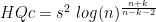
HQ stands for Hannan & Quinn, its inventors. SHIBATA and RICE are also named for their inventors.
GCV stands for Generalized Cross-Validation. Cross-validation, in general, refers to the idea of fitting an equation to a subset of the data, and then investigating how well it fits the rest of the data.
Reconciling the two equations for AIC
There are two other meaures I want to discuss, but first let’s reconcile my (and Ramanathan’s) simple formula for AIC,

with Mathematica’s formula:
![2+2 k+n+n Log[ESS/n]+n Log[2 \pi]](https://s0.wp.com/latex.php?latex=2%2B2+k%2Bn%2Bn+Log%5BESS%2Fn%5D%2Bn+Log%5B2+%5Cpi%5D&bg=ffffff&fg=000000&s=0&c=20201002)
Drop the three constant terms, getting
![2 k+n Log[ESS/n]](https://s0.wp.com/latex.php?latex=2+k%2Bn+Log%5BESS%2Fn%5D&bg=ffffff&fg=000000&s=0&c=20201002)
Subtracting constants will not change which regression has the minimum value. Of course, it will have a different value at the minimum, but if all I want is to know which regression has the minimum AIC, this is as good as the first expression.
Now divide by n. That will have no effect on where the minimum is, either, getting
![\frac{2k}{n}+Log[ESS/n]](https://s0.wp.com/latex.php?latex=%5Cfrac%7B2k%7D%7Bn%7D%2BLog%5BESS%2Fn%5D&bg=ffffff&fg=000000&s=0&c=20201002)
Now take the exponential. That’s a monotonic function, so it won’t move the minimum either.

And that’s my easy-to-use formula for AIC.
Oh, one other piece of business. If you read the Mathematica help system, it will say that the (k+1) term is the number of parameters to be estimated.
But I thought that was k.
Ah. The number of parameters in the fitted model is indeed k, the number of
Similar algebra will reconcile BIC as Mathematica computes it and as I compute it. And similar algebra will reconcile other expressions in McQuarrie & Tsai with their counterparts in Ramanathan (and my code).
Oh, since TSS depends only on the y’s, and n is a constant, we see that the Adjusted R Squared could have been manipulated to another form which would have a different maximum value but at the same place.
1 – s^2,
which makes it clear that it and s^2 (SIGMASQ) go inversely.
Maybe I should remove s^2 from my list of measures: it really is redundant. I have read that most of the others are not redundant, but I don’t know about all of them.
PRESS and Mallows’ Cp
Ok. What are the two other measures that I know how to compute?
One, like GCV, is a measure of cross-validation. What if we fit the equation to all but one point? But which point? Why not all of them?
Compute the deletion residuals (which I introduced here)

Compute the sum of squares, and call it PRESS (Partial Regression ESS):
PRESS = ed.ed
(No, I don’t know why we don’t divide by n-k. But if we divide by n, the resulting statistic is called CV(1), for “cross-validation dropping 1 observation”.)
Easy enough.
That leaves one more: Mallow’s Cp. It differs from all the others in that it requires two regressions; one is a touchstone against which all the others are compared.
We compute the measure in two steps. First, the actual Cp is given by
Cp = ESS / s^2 – (n-2k),
where s^2, however, is the estimated variance of our touchstone regression, but ESS and k come from the specific regression for which we are computing the Cp.
Second, what we want is that regression having the minimum value of
|Cp – k|.
That’s it: we want the regression having Cp closest to k, without regard to sign. (Mallows published the Cp is the early 1970s; in 1995 he suggested that any regression with Cp < k would be worth consideration. But that's not as convenient as minimizing |Cp – k|).
OK, that's how it's computed. But there's one other important consideration.
Look back at the equation for Cp, and suppose we are computing for the touchstone regression. Now we have s^2 = ESS / (n-k) and we get
Cp = n-k – n + 2k = k.
That is, for our touchstone, Cp = k, so |Cp – k| = 0. Cp tells us nothing useful about the touchstone. We want the minimum value of |Cp – k| for all of the regressions except the touchstone.
So we can't learn anything about our touchstone. So it better not be any of the regressions we care about!
In the case of the Hald data, our touchstone will usually be the regression using all 4 variables, and every other measure I compute will tell me that the touchstone is not a candidate for the "best regression".
What bothers me isn't so much that I can't apply Cp to the touchstone, but that the touchstone needs to be a poor enough fit that I don't care to test it.
This won't stop me from computing Cp, but for some of what I do, it won't really be very useful or accurate.
Generalizing AIC and FPE again
In addition to all these, there are two infinite families of measures which I did not use. If we write
then we could consider it a special case (with 

Similarly, we could define

(No, that doesn’t simplify to FPE when (

differs from

by
Huh?

As I said, I did not attempt to use these two infinite families of selection criteria. I wonder if there’s some value of 
In the next post, I’m going to look at regressions using every possible subset of the Hald variables, and we’ll see what these selection criteria tell us.

January 9, 2011 at 1:39 pm
In a comment under Suggestions, JEP said:
Hi JEP,
I’m glad to have been of help. And I wouldn’t mind at all if you cited my presentation of the two equations as confirmation of what Mathematica computes.
My source for the AIC formula was McQuarrie & Tsai, “Regression and Time Series Model Selection”, 981-02-3242-X, p. 21. I modified their SIC (BIC) formula on p. 23 by using (k+1) where they used k.
Then i confirmed that my two equations matched Mathematica’s answers. Mathematica’s brief discussion of AIC and BIC can be found in the tutorial for statistical model analysis, but I do not recall seeing the actual equations anywhere on Wolfram.
BTW, I’m going to copy this comment to the “selection criteria” post, as well as leaving the original under Suggestions.
rip