PCA / FA . “Preprocessing”

When I moved beyond the first couple of books, I was bewildered by the huge number of alternatives for PCA / FA. I think my final count was that there were 288 different ways of doing it. It was so bad that I put together a form so that whenever I read a new example I could check off boxes for the choices made. As I’ve gotten more experience, I no longer need that checklist.

A lot of those choices pertained to the starting point. If the analysis began with an eigendecomposition, well, it could have been applied to the correlation matrix, or to the covariance matrix – oh, and one text used N instead of N-1 to compute sample variances.

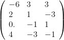
Or an eigendecomposition could have been applied to or to or to both… but X itself could have been raw data, centered data, doubly-centered data, standardized data, or small standard deviates. Oh, and X could have observations in rows (jolliffe, Davis, and I) or in columns (Harman). Oh boy.

Or we could have done an SVD of X, where X itself could have been raw data, centered data, doubly-centered data, standardized data, or small standard deviates, with observations in rows or columns. Yikes!

(not to mention that the data could very likely have been manipulated even before these possible transformations.)

Then I decided that all those choices were pre-processing, not really part of PCA / FA. Actually, I decided that I must have been careless, and missed the point when everyone made it, that one had to decide what pre-processing to do before starting PCA / FA. I was kicking myself a bit.

PCA / FA example 4: davis. Summary.

Considering how much I learned from Davis’ little example, I almost hate to summarize it. The following just does not do justice to it. We’ll see if the passage of time – coming back to Davis with fresh eyes after doing the next example – improves the summary.

OTOH, an awful lot of what I got out of Davis came from bringing linear algebra to it, and just plain mucking about with the matrices. And I discovered, having picked up the two chemistry books since I drafted this post, that they made a lot more sense than when I first looked at them. I have learned a lot from working with Davis’ example.

Here’s what I have. My own strong preference, but I’d call it a personal choice, is to use the SVD of the data matrix X:

and compute the A’s and S’s (R-mode and Q-mode loadings and scores):

.

.

.

.

Those equations are worth having as a conceptual basis even if one chooses to do eigendecompositions of or instead of the SVD.

PCA / FA example 4: davis. Davis & Jolliffe.

What tools did jolliffe give us (that i could confirm)?

1. Z = X A, A orthogonal, X old data variables in columns
2. serious rounding
3. plot data wrt first two PCs
4. how many variables to keep?

but jolliffe would have used the correlation matrix. Before we do anything else, let’s get the correlation matrix for davis’ example. Recall the centered data X:

i compute its correlation matrix:

Now get an eigendecomposition of the correlation matrix; i called the eigenvalues and the eigenvector matrix A. Here’s A:

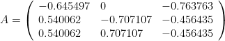
If we compute and get an identity matrix, then A is orthogonal. (it is.)

PCA / FA example 4: davis. Reciprocal basis 4.

(this has nothing to do with the covariance matrix of X; we’re back with for the SVD of X.)

in the course of computing the reciprocal basis for my cut down

i came up with the following matrix:

now, is very well behaved. Its two columns are orthogonal to each other:

PCA / FA example 4: davis. Davis & harman 3.

Hey, since we have the reciprocal basis, we can project onto it to get the components wrt the basis. After all that work to show that the are the components wrt the reciprocal basis, we ought to find the components wrt the basis. And now we know that that’s just a projection onto the reciprocal basis: we want to compute X B.

Recall X:

Recall B:

The product is:

What are the column variances?

Does that surprise you?

PCA / FA example 4: davis. Reciprocal basis 2 & 3.

The reciprocal basis for A^R using explicit bases.

Here I go again, realizing that I’m being sloppy. i call

the second data vector, but of course, those are the components of the second data vector. a lot of us blur this distinction a lot of the time, between a vector and its components. So long as we work only with components, this isn’t an issue, but we’re about to write vectors. i wouldn’t go so far as to say that the whole point of matrix algebra is to let us blur that distinction, but it’s certainly a major reason why we do matrix algebra. but for now, let’s look at the linear algebra, distinquishing between vectors and their components.

i need a name for the second data vector; let’s call it s. we will write it two ways, with respect to two bases, and show that the two ways are equivalent.

PCA / FA example 4: davis. Scores & reciprocal basis 1.

The reciprocal basis for , using matrix multiplication.

i keep emphasizing that is the new data wrt the orthogonal eigenvector matrix; and i hope i’ve said that the R-mode scores are not the new data wrt the weighted eigenvector matrix . In a very real sense, the R-mode scores do not correspond to the R-mode loadings . This is important enough that i want to work out the linear algebra. In fact, i’ll work it out thrice. (And i’m going to do it differently from the original demonstration that is the new data wrt v.)

Of course, people will expect us compute the scores , and I’ll be perfectly happy to. I just won’t let anyone tell me they correspond to the .

First off, we have been viewing the original data as vectors wrt an orthonormal basis. Recall the design matrix:

Let’s take just the second observation:

Those are the components of a vector.

Happenings – 21 Apr

We all know it’s been a while since I posted.

For one thing, last weekend I was working on the most important applied mathematics of the year: my income taxes. When they were done in principle (Friday evening), I went out and bought 4 DVDs and some chips and dip, and watched movies for a while.

Monday, I was at a friend’s, doing some Mathematica and some quantum mechanics.

Instead of doing a little bit of a lot of things, last weekend and this weekend, I focused on PCA / FA for the blog. I’ve done almost no other math. There were a bunch of PCA / FA things that just seemed like they should all be done before I started publishing any of them.

Technical posts on PCA / FA went out yesterday and today. More importantly, if you’re following that subject, there are 8 more posts ready to go: all I have to do is hit the “publish” button. I expect to put out one a day, no more. That may be overwhelming as it is.

Not exactly a steady pace, but there it is.

PCA / FA example 4: davis. Davis & harman 2.

What about redistributing the variance?

We learned from harman that if we use the orthogonal eigenvector matrix v to compute new data, the result has redistributed the original variance according to the eigenvalues; and we also learned that if we use the weighted eigenvector matrix instead, we get new variables of unit variance.

(i think i thought this required us to start with the correlation matrix; it does not.)

let’s see this again for davis’ centered data X:

We have variances…

or…

and the sum of the variances is…

32.

PCA / FA example 4: davis. Davis & harman 1.

Let us now recall what we saw harman do. Does he have anything to add to what we saw davis do? if we’re building a toolbox for PCA / FA, we need to see if harman gave us any additional tools.

here’s what harman did or got us to do:

• a plot of old variables in terms of the first two new ones
• redistribute the variance of the original variables
• his model, written Z = A F, was (old data, variables in rows) = (some eigenvector matrix) x (new data)

We should remind ourselves, however, that harman used an eigendecomposition of the correlation matrix; and the eigenvectors of the correlation matrix are not linearly related to the eigenvectors of the covariance matrix (or, equivalently, of .) having said that, i’m going to go ahead and apply harman’s tools to the davis results. i will work from the correlation matrix when we get to jolliffe.

What exactly was that graph of harman’s? he took the first two columns of the weighted eigenvector matrix, then plotted each row as a point. He had 5 original variables. His plot

shows that the old 1st and 3rd variables, for example, are defined very similarly in terms of the first two new variables. let me emphasize that this is a description of defining variables, not a display of the resulting data. Simple counting can help with the distinction, e.g. 3 variables but 4 observations.